Raster Analysis

Goal

The goal of this assignment is to use multiple raster geoprocessing tools to build a model for both suitable sand mining locations and environmentally risky locations in Trempealeau County, Wisconsin.


Objectives

This assignment is in two partitions. The first involves creating a sand mining suitability model based on five criteria:

1. Elevation
2. Land use/Land cover
3. Distance to railroads
4. Slope
5. Water-table depth

The second partition looks at the impact of sand mines on the environment based on the following six criteria:

1. Proximity to streams
2. Prime farmland
3. Proximity to residential areas
4. Proximity to schools
5. Visibility from prime recreational areas
6. Proximity to wildlife habitats

Sources and Datasets

Several datasets were used in this assignment:

The georeferenced bedrock geology map used in Objective 1 was obtained from the university's database. The digital elevation model (DEM for Objectives 1, 4, 12) and National Land Cover Dataset (NLCD for Objective 2) were obtained from the USGS. The rail terminals feature class (Objective 3) was obtained from the National Atlas. The water-table elevation map used in Objective 5 was obtained from the Wisconsin Geological Survey. The DNR Hydro (Objective 8), prime farmland (Objective 9), Parks (Objective 10), and Wildlife Areas (Objective 12) feature classes were all obtained from the Trempealeau County Dataset.

Suitability

Objective 1

The first objective was finding suitable land based on the elevation criteria. A georeferenced bedrock geology map of west-central Wisconsin was used in conjunction with contour lines generated from a DEM of the area. After substantial use of the swipe tool to compare the geology map with the elevation I was able to estimate the elevation range for both the Jordan (gold) and Wonewoc (red) formations. These two formations were stated in the lab as the two most desirable geologic formations for frac sand mining. I estimated the Wonewoc formation to be from 250-310 meters, and the Jordan formation to be from 330-370. With these two ranges in mind I did my first reclassify, which I did not feel turned out quite right, as I felt this resulted in the Wonewoc formation showing in too much area that it definitely was not (Figure 1). So, I decided to do a second reclassification, changing only the minimum of the Wonewoc range from 250 to 260. The resulting reclass can be seen in Figure 2. After examining the second reclassification, I felt it resulted in a greater amount of inaccuracy in the southern part of the county than increased accuracy in the northern portion, so I decided to stick with the first reclassification.

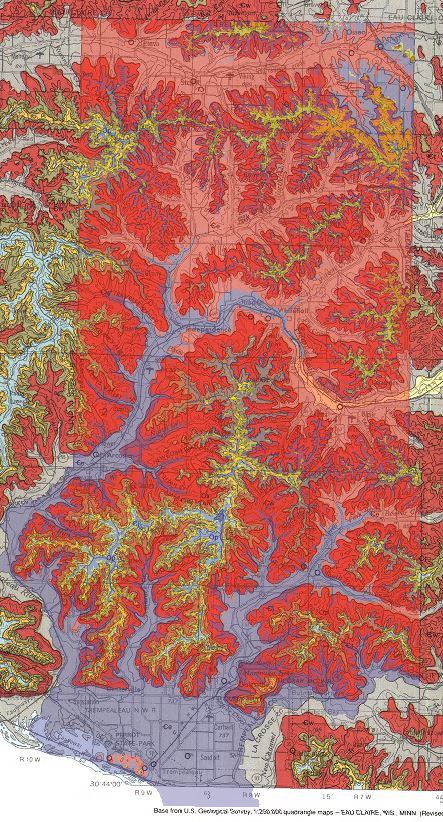Figure 1: The first reclass overlayed on the
georeferenced bedrock map.  In the northern
part of the county, you can see much of the
valley area is not in blue.

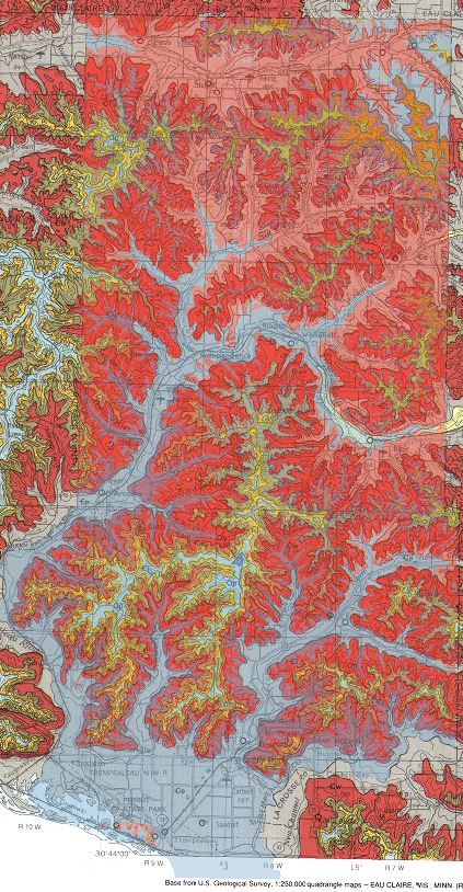Figure 2: This second image was an attempt
to increase the accuracy of the northern part
of the county.  Unfortunately, not very much
was gained, but the southern part of the county
became a bit more inaccurate.

The following criteria ranking was used in this objective:

3 – Wonewoc and Jordan formations, since these are the most suitable locations
2 – Elevations between the wonewoc and Jordan formations, as this is small range and between the two ideal
1 – Elevations above and below the Wonewoc and Jordan formations, as these are most unsuitable.


Objective 2

The second objective involves finding suitable land based on land use criteria. Using a land use/land cover dataset obtained from the NLCD. Using the NLCD 2001 legend found here, I was able to determine what the numbers in the value field related to for land use. This objective requires two reclassifications. The first reclass ranks each value from 1 to 3, with 3 being the easiest to clear for the mine. The second reclass will be used in the raster calculator at the end of the suitability model to exclude those zones that are not useable at all, such as open water, developed space, and wetlands.

Figure 3: Image of table from Excel


Objective 3

Finding suitable land based on proximity to railroad terminals was the third objective. This should have been a rather simple process, as all that was required was to run the Euclidean Distance tool on the rail terminals feature class, and then reclassify the distances into three ranks, 3 being the closest. This was not so simple due to the euclidean distance raster being clipped and not covering all areas of Trempealeau county (when Trempealeau county boundary was used as mask it registered the whole county as the same distance). To circumvent this I had to create a large mask layer in the same projection around the area I wanted to be calculated. Once I created the layer and set it as the mask in the Environments settings, all was good.

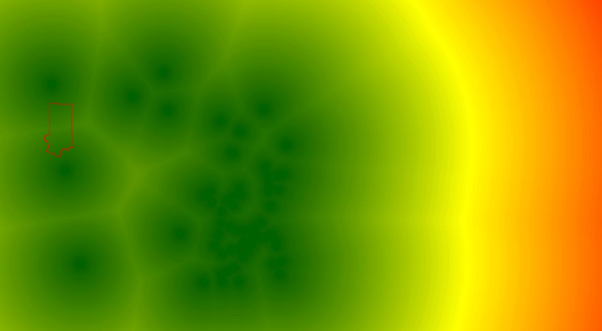Figure 4: Screenshot of the euclidean distance ran and the size of the mask. My first mask

attempt was a square around Trempealeau county, but it did not work properly for

unknown reasons, so I created this one.  As you can see, the Euclidean Distance
goes far beyond Trempealeau County (outlined in red).

Objective 4

The same DEM from Objective 1 is used in this objective to determine the slope. The slope tool was ran with the output measurement parameter set to percent rise. The percent rise is a mathematical equation used to describe the slope of terrain, streets, roads, etc., with 100% rise being equivalent to a 45 degree angle. The focal statistics tool was then used to average the slope values to limit the “salt and pepper effect,” which is when pixels are erroneously ascribed the minimum or maximum value. A rectangular (3 cell by 3 cell) neighborhood and the mean statistics were used as parameters for the focal statistics tool. The resulting raster was then reclassified to the values seen in Figure 5.

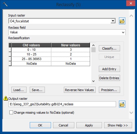Figure 5: This is the Reclassify tool.  As you can see, all cells with values 0-10 will
be converted to 3, 10-25 will become 2, and above 25 will be 1.

Objective 5

Since the mined sand needs to be washed to remove fine particles, the ideal location of a mine requires the water table to be as close to the surface as possible. After downloading the water-table elevation map from the Wisconsin Geological Survey, the coverage file was projected and then converted to a raster using the Topo to Raster tool and the WT_ELEV field of the contours layer. With the water-table as a raster, it was then reclassified, with the closest to the surface being 3, and the further it was away would be 2, and then 1.


Objective 6 and 7

While objective six used the raster calculator to add all of the reclassifications, objective seven removed the exclusion zones by multiplying the raster calculator by the exclusion reclass. I decided to do both of these in a single calculation (Figure 6). In Figure 7, you can see the model used for the suitability assessment. All of the reclassifications can be seen in a Figure 8, and the final suitability model is shown in Figure 9.

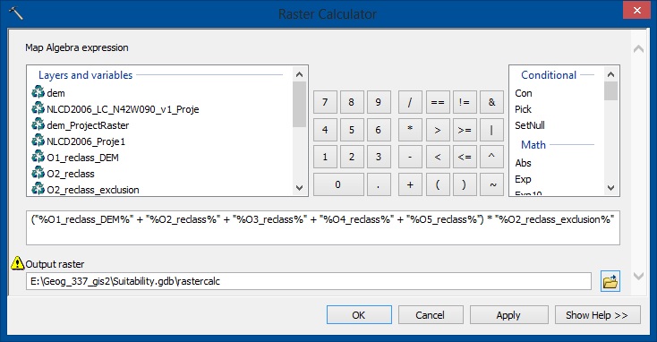Figure 6: This screenshot shows the equation used to generate the map.
As you can see, it simply adds all of the rasters together, and then
multiplies them by the exclusion raster.

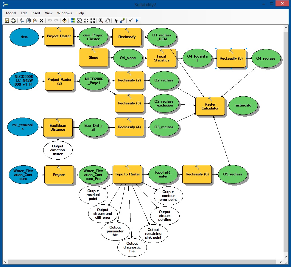Figure 7: This is the model I created using ModelBuilder in ArcMap.
Almost all of my processes were ran through model builder.

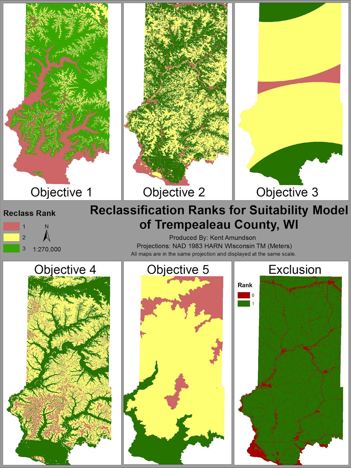Figure 8: This image shows the resulting map for each objective
in the Suitability Model.

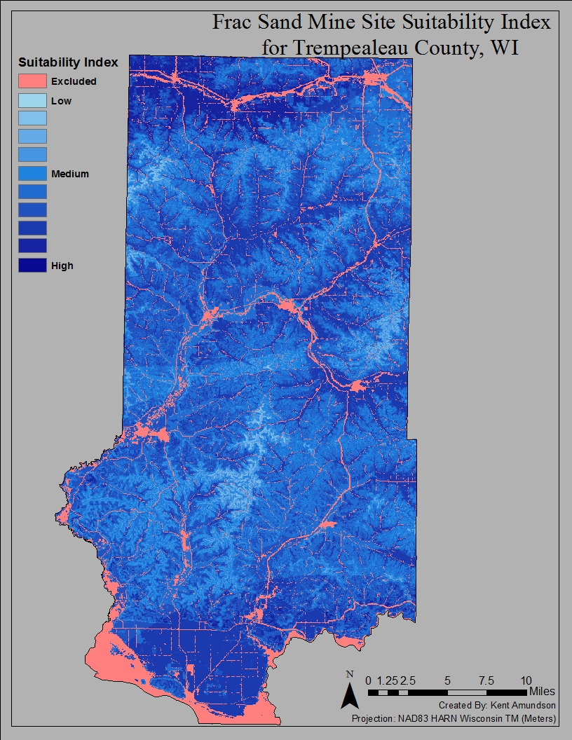Figure 9: The final Suitability map generated from running the
Raster Calculator tool.  Using the equation found in Figure 6
resulted in this map.

Risk Assessment

For the risk assessment portion of this analysis, each objective will also use the Reclassify tool to create three ranks that represent the amount of environment risk in that area. A 3 will represent high environmental risk, 2 will be medium risk, and 1 will represent a low risk location. A single map in the final objective will show the map of each objective (Figure 11).

Objective 8

Objective eight used the Euclidean Distance tool to measure the distance land was from rivers. I classified areas within an eighth of a mile of rivers as a 3, areas between an eighth and half a mile as a 2, and beyond that as a 1. While there appears to be very few, if any, substantial impacts to rivers as a result of the mining process, these ranges were used to increase the distance, just in case.


Objective 9

Since Wisconsin is a large agricultural state, it would be very unfortunate to lose prime farmland to sand mines. With this in mind, a prime farmland feature class was converted to a raster, and then reclassified based on the attributes of each cell. If the land was prime farmland, is was classified as a 3. If it could be considered prime farmland if it was either drained or protected from flooding, it was classified as a 2. All other land was classified as low risk, 1.


Objective 10

Another issue with local communities and neighborhoods around sand mines is the potential dust and noise generated by the mining process. To reduce these issues, a sand mine must be at least 640 meters away from residential or populated areas. I used a composite boundaries feature class, and selected all of the areas considered to be city limits, then used the Euclidean Distance tool to measure the distances of each cell from those areas. Distances up to 640 meters were reclassified as high risk, those from 640 meters to 2 kilometers as medium risk, and everything beyond that was low risk.


Objective 11

Though most schools should have been included by using the city limits in the previous objective, it is important to be certain. For this reason, parcel data of the county was used, and all parcels owned by a school district were selected and the Euclidean Distance tool was used. The same classifications were used as in objective ten.


Objective 12

It would be quite sad if our beautiful parks and the views of nature they provided were restricted by the obvious sand mine off in the distance, so the Viewshed tool was used to find the areas of land that were visible from recreational areas. Two viewsheds were intended to be done, one on the parks and another on the trails, but technical issues arose, resulting in only one being completed. Using the DEM as the input raster, and the parks feature class as the observer feature, a viewshed was completed after about 15 minutes of processing time. Visible areas were classified as high risk, and all other areas were classified as no risk (0). The trails viewshed was attempted, but after six hours of processing time it was at only 8% completion and so was aborted.


Objective 13

The final factor before risk calculation was of my own choice. I decided that wildlife areas should be preserved as well, as I believe potential loss of wildlife is of environmental importance as well. As a result, I used a wildlife areas feature class and, again, ran the Euclidean Distance tool. I then reclassified the areas based using the same distances as objectives ten and eleven.


Objective 14

In this final objective, Raster Calculator was used to generate a map of the risk assessment for Trempealeau County, Wisconsin. Figure 10 shows the equation used to generate this map. In Figure 11 you can see the maps generated in each objective and the Risk Index used. The model created and used in ModelBuilder can be seen in Figure 12, while the final risk assessment map can be seen in Figure 13.

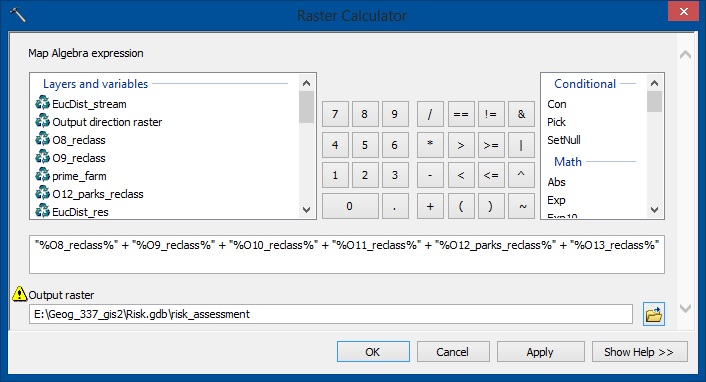Figure 10: This screenshot shows the equation used to
generate the Risk Assessment Map.  As can be seen, it is
simply the sum of all the reclassifications.

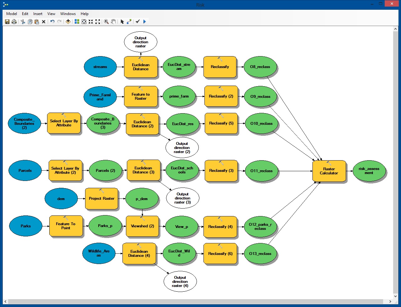Figure 11: This is a screenshot of my Risk Model built using
ModelBuilder in ArcMap.  All tools were run using this model.

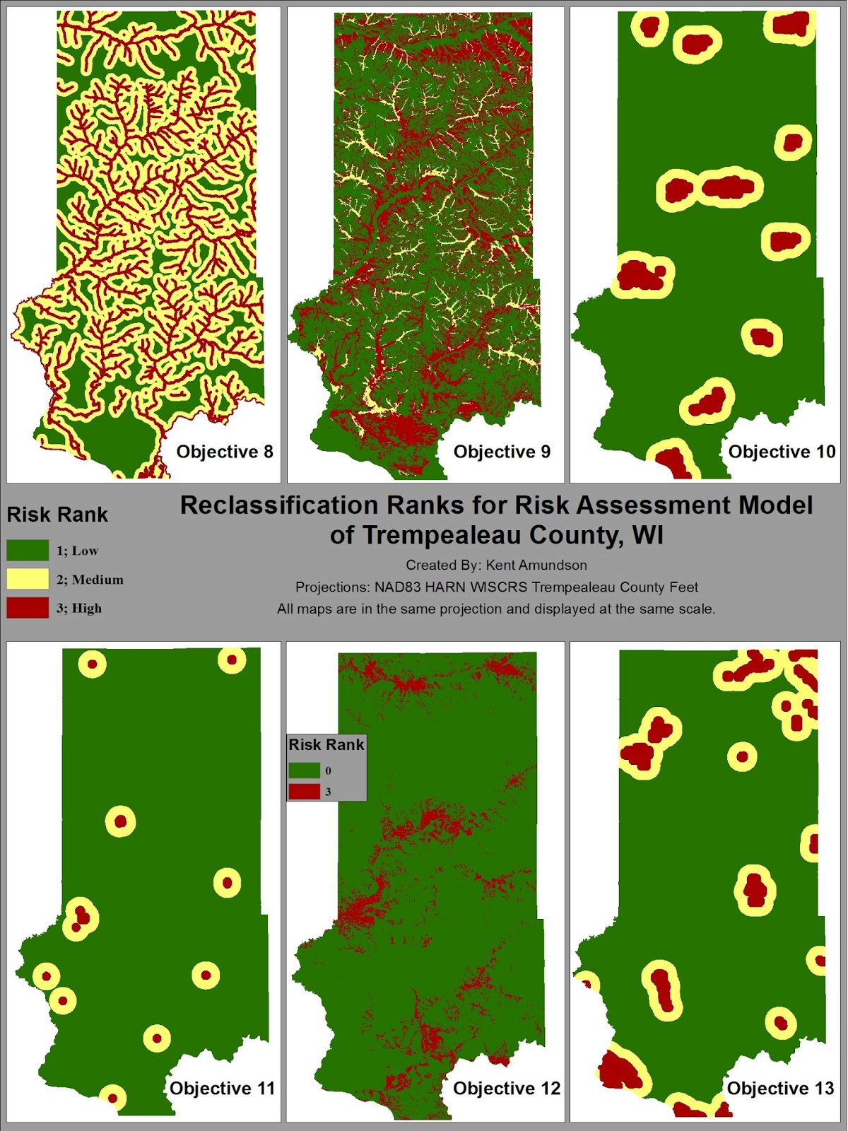Figure 12: The maps generated in each objective can be seen
in this image.  

Figure 13: This is the environmental risk assessment map
generated by the raster calculator equation in
Figure 10.

Conclusion

Through this raster analysis two maps of use have been generated, one indicating the most suitable locations for mines, and one establishing the areas of greatest environmental risk.  Neither of them can be used alone without potentially causing issues.  If only the Suitability map were used, then a mine could be built without taking into account the environmental risks associated with that location.  For that reason, I created another map (Figure 14).  This map was created using the raster calculator to subtract the Risk Index from the Suitability Index, meaning each cell value in the Suitability Map would be subtracted by that same cells value in the Risk Map.  The resulting raster had cell values ranging from -17 to 10.

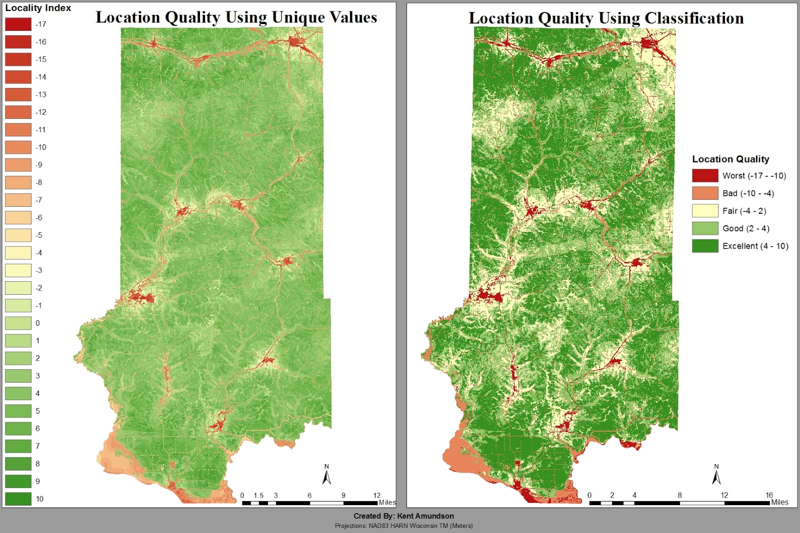Figure 14: Two maps using two different methods in the Symbology tab.  These maps were generated using the
Raster Calculator.  The Risk Index was subtracted from the Suitability Index, resulting in cell values ranging
from -17 to 10.  The classification on the map on the right was done using natural breaks (Jenks).